Getting started

This tutorial will guide you through installing the required libraries for the rest of the tutorials, downloading and accessing the dataset, and loading some data to view.

Setup your environment

A full list of required packages are defined in a conda environment.yml file. For the purposes of this tutorial, we will only install the required dependencies. You may skip this step if you’re an existing environment.

!pip install nilearn mne mne_bids

Now that the libraries are installed, we will load them.

import mne
import numpy as np
from mne_bids import BIDSPath

Download the data

For this tutorial, we will download one file from the dataset. To download the entire dataset, see the how to download page.

Because the dataset is structured according to BIDS conventions, we can use the BIDSPath class to define the path components and construct a path. For simplificty, we will load the preprocessed ECoG data from the dataset. This file exists under the derivatives/ecogprep/ directory, and has the name sub-0*_task-podcast_desc-highgamma_ieeg.fif. The fif extension signifies this is an MNE format that contains the data and metadata in one file.

file_path = BIDSPath(root="derivatives/ecogprep",
                     subject="02",
                     task="podcast",
                     datatype="ieeg",
                     description="highgamma",
                     suffix="ieeg",
                     extension="fif")
print(f"File path within the dataset: {file_path}")

File path within the dataset: derivatives/ecogprep/sub-02/ieeg/sub-02_task-podcast_desc-highgamma_ieeg.fif

Now we can download the file using wget:

!wget -nc https://s3.amazonaws.com/openneuro.org/ds005574/$file_path

File ‘sub-02_task-podcast_desc-highgamma_ieeg.fif’ already there; not retrieving.

Verify dataset

Now that we have the dependencies installed and the data file downloaded, we’ll load it using the MNE library. We’ll be using MNE throughout the tutorials. To load the data file we downloaded, we’ll use the read_raw_fif function, and then display some of the metadata about the file.

raw = mne.io.read_raw_fif(file_path.basename, verbose=False)
raw

	General
	Filename(s)	sub-02_task-podcast_desc-highgamma_ieeg.fif
	MNE object type	Raw
	Measurement date	2001-01-01 at 01:01:01 UTC
	Participant	sub-02
	Experimenter	Unknown
	Acquisition
	Duration	00:29:60 (HH:MM:SS)
	Sampling frequency	512.00 Hz
	Time points	921,600
	Channels
	ECoG	90
	Head & sensor digitization	93 points
	Filters
	Highpass	70.00 Hz
	Lowpass	200.00 Hz

The output contains several important pieces of information. First, duration of the data is roughly 30 minutes long (corresponding to the length of the podcast). The data is sampled at 512 Hz. There are 90 ECoG channels. And the data has a filtered applied to it ranging from 70 Hz to 200 Hz.

One of the primary MNE classes is the Raw. It has many useful methods and properties if you look at its documentation. The two we will mention now are get_data() and the info attribute. Sometimes we want to work with the underlying data directly. Here is how:

data = raw.get_data()
print(f"Data is a {type(data)} object and has a shape of: {data.shape}")

Data is a <class 'numpy.ndarray'> object and has a shape of: (90, 921600)

We notice that the data is a NumPy object (a nearly universal way of working with numerical data in python), and its a matrix with two dimensions. The first dimension corresponds to the number of channels—90, as we saw before— and the second is the total number of samples.

raw.info returns an Info object. We saw this information earlier as it contains much of the metadata of the file. Particularly useful are the information we can get on those 90 channels. This can be accessed by raw.info.ch_names and raw.info.chs. The documentation spells out the details very clearly. Below, we’ll use the channel information to get electrode locations and plot them on a brain.

For example, let’s look at just the first electrode.

print("First channel name is:", raw.info.ch_names[0])
print("Metadata associated with the first channel:")
raw.info['chs'][0]

First channel name is: PO1
Metadata associated with the first channel:

{'scanno': 1,
 'logno': 1,
 'kind': 902 (FIFFV_ECOG_CH),
 'range': 1.0,
 'cal': 1.0,
 'coil_type': 1 (FIFFV_COIL_EEG),
 'loc': array([-0.06466667, -0.051     , -0.01066667,  0.        ,  0.        ,
         0.        ,         nan,         nan,         nan,         nan,
                nan,         nan]),
 'unit': 107 (FIFF_UNIT_V),
 'unit_mul': 0 (FIFF_UNITM_NONE),
 'ch_name': 'PO1',
 'coord_frame': 4 (FIFFV_COORD_HEAD)}

The loc key in the dictionary gives us the 3D coordinates (x, y, and z) that localize the electrode in brain space.

Ploting electrodes on the brain

Now we’ll use a library called nilearn to help us plot the electrodes on a glass brain. We’ll be using the function plot_markers. Take a quick look at its parameters in the documentation, as they can be very useful.

from nilearn.plotting import plot_markers

At a minimum, this function requires a set of values, and a corresponding set of coordinates. The coordinates tell nilearn where to plot the electrode, while the value tells it what color to assign it. For the example below, we just want to plot them all in one color, so values will be all the same number. Importantly, we need to collate the coordinates into a NumPy matrix of shape (n, 3) where n is the number of electrodes and the 3 columns are the coordinates of each electrode. First, we’ll assemble this matrix:

ch2loc = {ch['ch_name']: ch['loc'][:3] for ch in raw.info['chs']}
coords = np.vstack([ch2loc[ch] for ch in raw.info['ch_names']])
coords *= 1000  # nilearn likes to plot in meters, not mm
print("Coordinate matrix shape: ", coords.shape)

Coordinate matrix shape:  (90, 3)

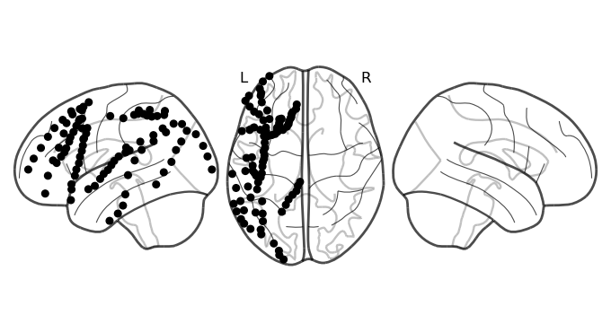
And now we plot them on the brain:

values = np.ones(len(coords))
fig = plot_markers(values, coords,
             node_size=30, display_mode='lzr', alpha=1,
             node_cmap='Grays', colorbar=False, node_vmin=0, node_vmax=1)
print(fig)

<nilearn.plotting.displays._projectors.LZRProjector object at 0x1454e3ff2a50>